The Database Menu: SQL vs NoSQL, Explained Like You're New

Every backend project reaches the same question sooner or later: which database should we use? The useful answer is that it depends on three things: what you're storing, how you'll read it, and how much of it there is. SQL and NoSQL databases are different sets of tradeoffs rather than rival teams, and each one is excellent at some jobs and painful at others.

This post walks the menu the way you'd actually use it. If you're new, Sections 1 and 2 assume no background, every term is defined the first time it appears, and each section has diagrams with a note on how to read them. Section 3 goes inside a SQL database to cover isolation levels, the part of ACID that surprises experienced engineers most often, and the part the previous post (#15) promised. Section 4 covers the four NoSQL families, Section 5 is how each kind scales, and Section 6 explains CAP and its more useful cousin, PACELC. Section 7 is where each choice bites, Section 8 has the numbers and a decision framework, and Section 9 is the principal-level view: why real systems run several databases, and how to keep them from drifting apart. The one-page summary is at the end, under The database menu, distilled.

---

Section 1: Two families, one question

There are two broad philosophies about storing data.

SQL databases, also called relational databases (PostgreSQL, MySQL, SQL Server, Oracle, SQLite), store data in tables: rows and columns, like a very strict spreadsheet. Before you store anything, you declare the shape, called the schema: this table has a name column that holds text, an email column that must be unique, a created_at column that holds a timestamp. The database enforces that shape on every write. Try to put a phone number where a date belongs and it refuses.

NoSQL databases are everything that doesn't follow that model. The name is usually read as "not only SQL," and it covers several quite different designs that relax the table-and-schema rules to get something else in return, such as easier spreading across many machines or a data model that fits one kind of problem much better. Section 4 covers the four main families.

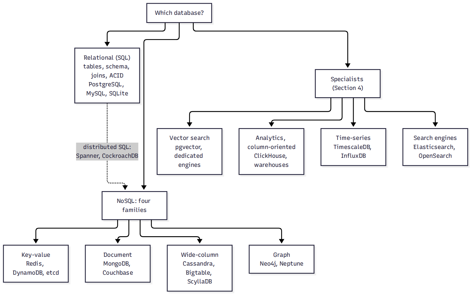
Figure 1. The menu this post walks through. The top split is the one people argue about, but the bottom row matters just as much in practice: many systems need a relational core plus one or two specialists. The dotted line is distributed SQL, which keeps the relational model while spreading data across machines the way NoSQL systems do (Section 5).

The choice matters because the database is the hardest part of a system to change later. You can swap a cache or add servers in an afternoon. Moving a terabyte of live data from one database to another, with traffic running the whole time, is usually a project of months, with real risk of an outage along the way. That makes it worth reading the menu carefully before you order.

---

Section 2: SQL, the strict spreadsheet that earned its keep

A SQL database thinks in tables and the relationships between them. A users table, an orders table, and each order row holding a user_id that references a row in users, which is called a foreign key. The database can enforce that relationship, so an order can never point to a user who doesn't exist. You query it in SQL, a language that has been around since the 1970s and is the closest thing the industry has to a universal query language: learn it once and it works on Postgres, MySQL, SQLite, and most analytics databases too.

SQL's strength is that you can ask questions you didn't plan for. "Revenue by country for customers who signed up last spring and bought more than twice" is a JOIN (a query that combines rows from several tables on matching keys) plus some filters and a GROUP BY, and the database works out how to answer it. What makes that fast is the index: a separate, sorted structure, usually a B-tree (a shallow, wide tree that finds any key in a few disk reads), that maps column values to the rows that hold them, so the database can jump to matching rows instead of reading the whole table. Indexes aren't free. Each one is updated on every write, which is why a heavily indexed table writes more slowly.

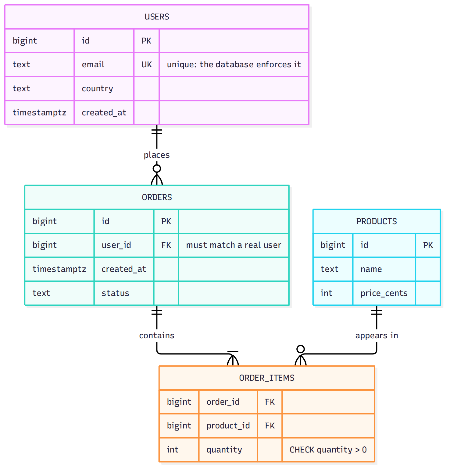
Figure 2. A small relational schema. Each box is a table, and each line is a foreign key the database enforces: an order can't reference a user who doesn't exist, and an order item can't reference a missing product. Because the relationships are declared, a question nobody planned for, like revenue by country for repeat buyers, is a query rather than a project.

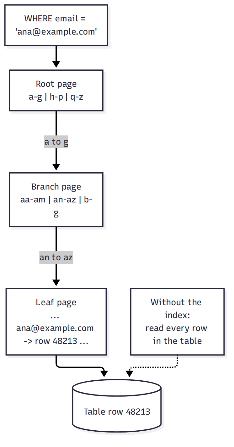
Figure 3. How a B-tree index finds one row. Each page splits the key range, so even a table with a billion rows needs only a handful of page reads to reach the right leaf, which points at the row. The dotted path is the alternative, a full table scan. Every index also has to be updated on every insert, which is the write cost mentioned above.

Its other strength is correctness, summarized by the acronym ACID, which #15 covers in depth:

• Atomicity: a transaction (a group of changes treated as one unit) either fully happens or doesn't happen at all.
• Consistency: declared rules, like unique emails or non-negative balances, hold before and after every transaction.
• Isolation: transactions running at the same time don't trip over each other's half-finished work. It comes in degrees, and Section 3 is about those degrees.
• Durability: once the database confirms a commit, the data survives a crash, because the change was first recorded in the write-ahead log, a file where every change is written before it's applied.

How far does one SQL database go? Further than most people expect. In January 2026, OpenAI described running ChatGPT's main PostgreSQL workload, serving 800 million users, on a single primary database with nearly 50 read replicas (copies that serve reads, covered in #5), handling millions of queries per second (QPS) for read-heavy traffic. The same post explains where it stopped working, which Section 9 comes back to. Most companies never need anything bigger than one primary and a couple of replicas.

---

Section 3: Inside SQL: isolation levels and the anomalies they allow

"Isolation" sounds absolute, but it's a dial. Full isolation, where every transaction behaves as if it ran alone, one after another, is called serializable, and it costs throughput. So databases offer weaker levels, and each level allows certain anomalies, meaning specific ways concurrent transactions can see or produce results that no one-at-a-time ordering would.

The anomalies, from most to least obvious:

• Dirty read: you read another transaction's change before it commits, and then it rolls back. You acted on data that never existed.
• Non-repeatable read: you read a row twice in one transaction and get different values, because someone committed a change in between.
• Phantom read: you run the same query twice and get a different set of rows, because someone inserted or deleted matching rows in between.
• Lost update: two transactions read a value, both modify it, and both write it back, so one write silently overwrites the other. Two people incrementing a counter from 10 both write 11.
• Write skew: two transactions each read the same data, each make a decision based on it, and each write to different rows, so neither overwrites the other, yet together they break a rule. Kleppmann's example in Designing Data-Intensive Applications: a hospital requires at least one doctor on call; two doctors on call both check that someone else is still on call, both go off call at the same moment, and nobody is left.

The standard levels, from weakest to strongest, are read uncommitted, read committed, repeatable read, and serializable. What the defaults actually are is where people get caught:

• PostgreSQL defaults to read committed. Each statement sees data committed before that statement began, so non-repeatable reads and lost updates are possible unless you guard against them. Postgres treats read uncommitted as read committed. Its repeatable read is stronger than the SQL standard requires and also prevents phantoms. Its serializable level uses a technique called Serializable Snapshot Isolation, which detects dangerous patterns and aborts one of the transactions with a serialization failure (error code 40001), so your application must be ready to retry.
• MySQL's InnoDB engine defaults to repeatable read. Same name as a Postgres level, different behavior. A concrete case: two transactions read a balance, then both update it. In Postgres's repeatable read, the second update fails with error 40001 and must retry. In InnoDB's repeatable read, the UPDATE reads the latest committed row rather than the transaction's snapshot, so an application that computed the new balance from its earlier read silently loses the other update. "We use repeatable read" means little until you say which database.

PostgreSQL's documentation summarizes what each of its levels allows. "Possible" means your application has to guard against it:

Level in PostgreSQL	Dirty read	Non-repeatable read	Phantom read	Serialization anomaly (e.g. write skew)
Read uncommitted (behaves as read committed)	not possible	possible	possible	possible
Read committed (the default)	not possible	possible	possible	possible
Repeatable read	not possible	not possible	not possible in Postgres (the standard allows it)	possible
Serializable	not possible	not possible	not possible	not possible

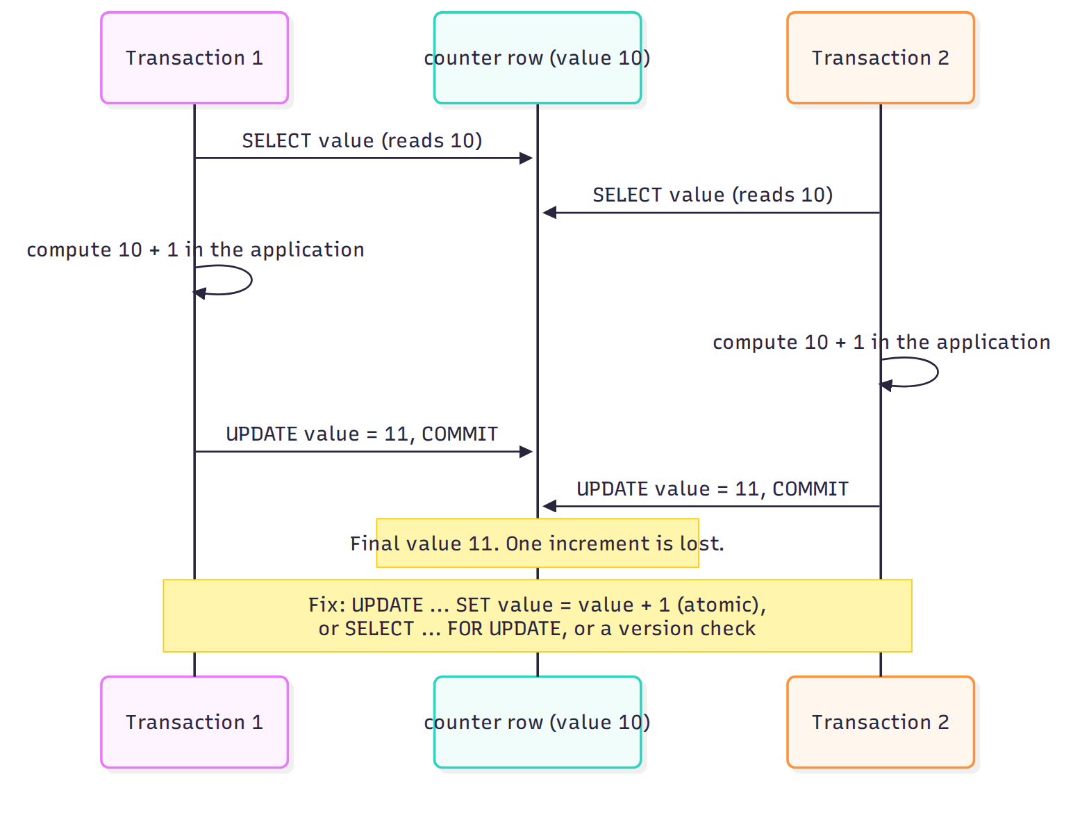
Figure 4. A lost update. Both transactions are individually correct, and neither sees an error; the bug is that each computed the new value from a read the other was about to make stale. The fixes in the note move the read and the write into one atomic step or make the second writer wait or fail.

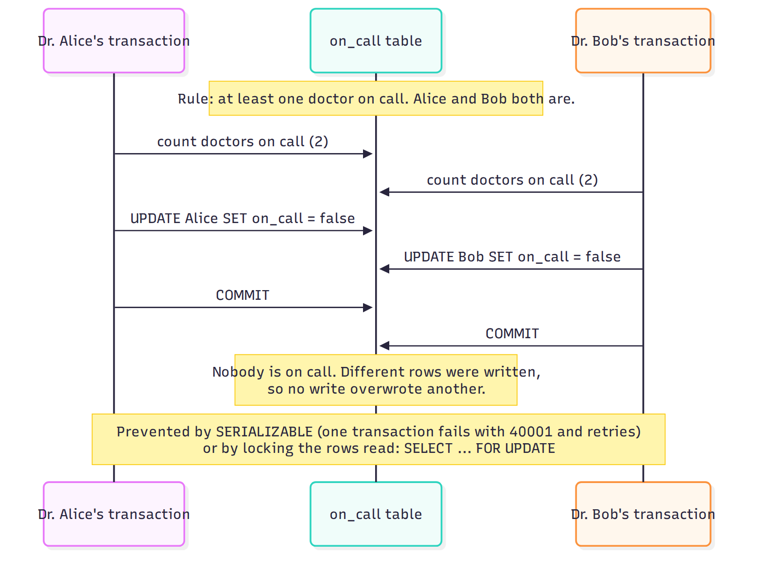
Figure 5. Write skew, using Kleppmann's on-call example. Unlike a lost update, the two transactions write different rows, so row locks on the written rows don't help. The rule they broke spans several rows, which is why only serializable isolation, or explicitly locking what you read, prevents it.

Both databases avoid most reader-writer blocking through MVCC, multi-version concurrency control: instead of overwriting a row in place, a write creates a new version of it, and each transaction reads the versions that were committed when its snapshot began. Readers don't block writers and writers don't block readers. The bill arrives later. In Postgres, every update writes a whole new row version and leaves the old one behind as a dead tuple until a background process called VACUUM cleans it up. OpenAI's 2026 post names exactly this, write amplification plus table and index bloat plus autovacuum tuning, as the main reason it moved write-heavy workloads elsewhere.

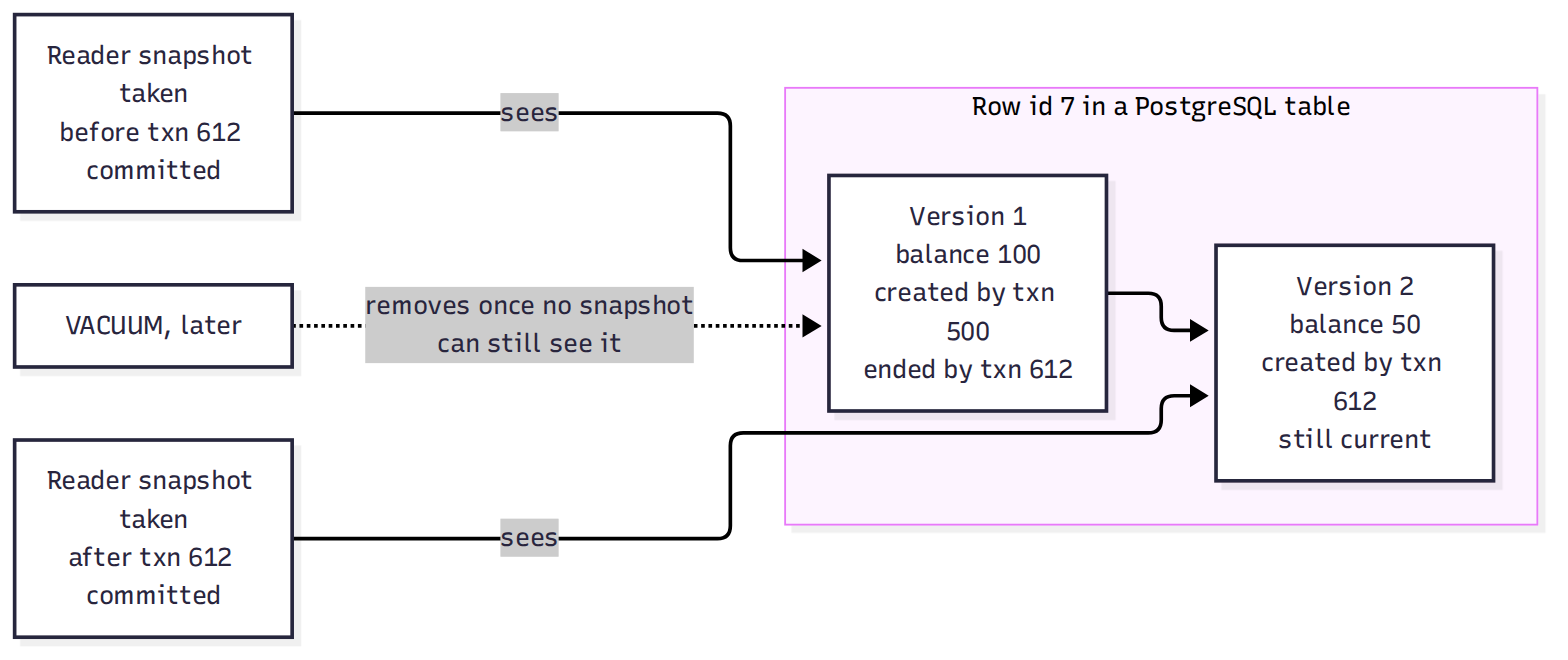
Figure 6. MVCC in one row. An update doesn't overwrite version 1; it writes version 2 and marks version 1 as ended. Each reader sees the version that matches its snapshot, which is why readers and writers don't block each other. The cost is the dead version left behind until VACUUM removes it, which is the write amplification and bloat OpenAI described.

What to do with all this:

1. Know your default. Most application bugs here come from assuming serializable while running read committed.
2. Fix lost updates in the query itself. UPDATE accounts SET balance = balance - 50 WHERE id = 7 is atomic; reading the balance into the application, subtracting, and writing it back is not. Alternatives are SELECT ... FOR UPDATE, which locks the row, or optimistic locking with a version column that each write checks and increments.
3. Use serializable for the few transactions where write skew would hurt, like scheduling, inventory, and money, and wrap them in a retry loop for 40001 errors.

---

Section 4: NoSQL, four families, four tradeoffs

NoSQL covers four different answers to the question "what if we dropped the tables?"

Key-value stores (Redis, Amazon DynamoDB, etcd) work like a giant dictionary: give it a key, get back a value. Redis keeps everything in memory and answers in well under a millisecond. DynamoDB is a managed service that spreads data across partitions by key and is built for single-digit-millisecond responses at almost any scale; Amazon reported it peaking at 151 million requests a second during Prime Day 2025. DynamoDB is richer than a pure dictionary, since items in one partition can be sorted by a second key and queried by range, and you can add secondary indexes. But the core rule holds: you must know the key, or have built an index for the question, before you ask. Key-value is the right answer when the access pattern is "I know exactly what I want": sessions, shopping carts, feature flags, counters, user profiles fetched by id.

Document stores (MongoDB, Couchbase) store JSON-like documents: nested, flexible, self-describing. A user document can hold its addresses and preferences inside it, so one read returns the whole thing. No schema is required up front; one user can have three addresses and another none. The tradeoff is that flexibility is a loan you repay later. Without the database enforcing a shape, your application code becomes the schema, and five services writing five slightly different shapes into one collection is a reliable source of bugs. Documents also have hard size limits: 16 mebibytes in MongoDB, and 400 kilobytes for a DynamoDB item.

Wide-column stores (Apache Cassandra, Google Bigtable, ScyllaDB) organize data into rows grouped by a partition key and sorted within each partition, spread across many machines. Cassandra and ScyllaDB have no single primary at all; any replica can accept a write. They were built to take enormous write volumes and keep running when machines fail. In 2011 Netflix benchmarked Cassandra on AWS at 1.1 million client writes a second on 288 nodes, which became 3.3 million writes a second once each write was copied to three availability zones (separate data centers within one cloud region). The tradeoff is a rigid query model: you design each table around one specific query, and questions you didn't design for, like an ad-hoc join, range from awkward to impossible. Consistency is tunable: per query, you choose how many replicas must respond, which Section 6 explains.

The reason wide-column stores write so fast is their storage engine. Most SQL databases keep data in a B-tree and update pages in place, which means random disk writes. Cassandra and similar systems use an LSM tree (log-structured merge tree): writes go to a sequential commit log and an in-memory sorted table (the memtable), get flushed to disk as immutable sorted files (SSTables, short for sorted string tables), and a background process called compaction merges those files over time, discarding overwritten data and tombstones (markers left by deletes, which Section 7 comes back to). Writes become cheap sequential appends. The cost moves to reads, which may check several files, and to compaction, which competes for disk and CPU and is behind many Cassandra performance incidents.

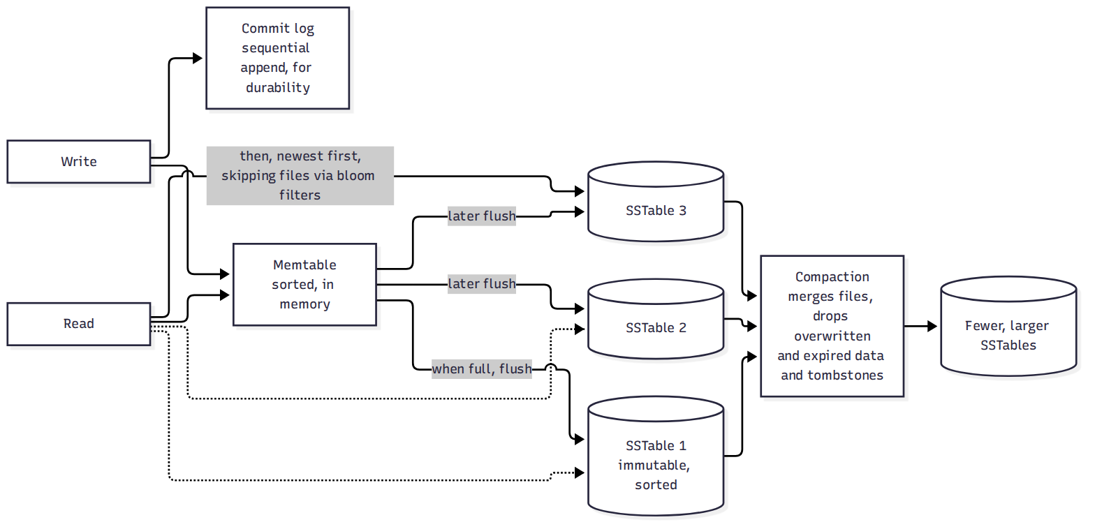
Figure 7. An LSM tree, the storage engine behind Cassandra and many other write-heavy stores. Writes only append to a log and update memory, so they're fast and sequential. Reads may have to check several files, which bloom filters (small structures that answer "definitely not here") keep cheap, and compaction does the deferred cleanup in the background, competing with live traffic for disk.

Graph databases (Neo4j, Amazon Neptune) store nodes and the relationships between them as first-class data. "Friends of friends who bought this" is a short walk across edges in a graph database, where in SQL it's a stack of self-joins. They're specialist tools. For general workloads they're slower and harder to scale than the generalists, and plenty of "we need a graph database" moments turn out to be handled fine by a well-indexed edges table and a recursive query (WITH RECURSIVE), until the traversals get deep or the graph gets huge.

Beyond the four families. Four kinds of specialist store show up on real menus in 2026, and each one is usually added next to a relational core rather than instead of it:

• Vector search. Machine-learning models turn text, images, or products into embeddings, lists of numbers placed so that similar things sit close together, and vector search finds the nearest neighbors of a query. Dedicated vector databases exist, but the pgvector extension adds this to PostgreSQL. Its documentation lists two index types. HNSW (Hierarchical Navigable Small World, a layered graph linking each vector to its near neighbors) "has better query performance than IVFFlat (in terms of speed-recall tradeoff)" but "has slower build times and uses more memory," while IVFFlat (an inverted-file index that groups vectors into clusters and searches only the nearest clusters) builds faster and uses less memory but queries more slowly. Both are approximate, meaning they trade a little recall (sometimes missing a true nearest neighbor) for speed. My default is pgvector until the vector count or query rate proves it isn't enough, because then embeddings live next to the rows they describe and can be filtered with ordinary SQL.
• Analytics. The databases in this post so far are built for OLTP (online transaction processing): many small reads and writes of individual rows. Analytics is OLAP (online analytical processing): a few huge queries that scan billions of rows but only a handful of columns. Column-oriented stores like ClickHouse, BigQuery, Snowflake, and Redshift store each column separately, so a query reads only the columns it needs, and similar values compress extremely well. They're poor at updating single rows, which is why they're fed from the transactional database rather than replacing it.
• Time-series. Metrics, sensor readings, and events keyed by time arrive in order, are rarely updated, and are usually queried by time range. Time-series databases (TimescaleDB, built as a PostgreSQL extension; InfluxDB; the storage inside Prometheus) build in time partitioning, compression, retention policies, and downsampling (keeping old data at lower resolution).
• Search engines. Elasticsearch and OpenSearch keep inverted indexes, maps from each word to the documents containing it, and rank results by relevance, which a B-tree can't do. Treat them as derived stores fed from your system of record, not as the system of record itself.

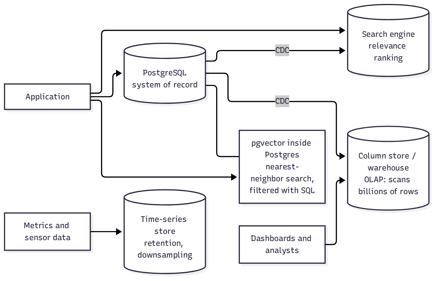
Figure 8. Where the specialists usually sit. The relational core holds the truth; the warehouse and search engine are fed from it by change data capture (Section 9); vector search often lives inside the core via pgvector; time-series data arrives on its own path. Each arrow is a copy that can lag, which is the cost of adding a specialist.

One feature, modeled both ways. The difference between "model your entities" and "model your queries" is easiest to see on one feature: show a customer their most recent orders. In SQL you model the entities and add an index for the query:

CREATE TABLE customers (id bigint PRIMARY KEY, name text NOT NULL);
CREATE TABLE orders (
  id           bigint PRIMARY KEY,
  customer_id  bigint NOT NULL REFERENCES customers(id),
  created_at   timestamptz NOT NULL,
  status       text NOT NULL,
  total_cents  int  NOT NULL
);
CREATE INDEX orders_by_customer ON orders (customer_id, created_at DESC);

-- The planned question: a customer's 20 most recent orders
SELECT * FROM orders WHERE customer_id = 123 ORDER BY created_at DESC LIMIT 20;

-- An unplanned question next month: pending orders older than an hour, any customer.
-- It runs today (perhaps slowly); add an index when it matters.
SELECT * FROM orders
 WHERE status = 'pending' AND created_at < now() - interval '1 hour';

In DynamoDB you design the keys around the question. AWS's own guide describes single-table design as storing several entity types in one table so that one request can fetch them together:

PK              SK                              attributes
CUSTOMER#123    PROFILE                         name = "Ana"
CUSTOMER#123    ORDER#2026-10-11T09:30#9001     status = pending, total = 5000
CUSTOMER#123    ORDER#2026-10-02T14:05#8812     status = shipped, total = 1200

Planned question, one request, newest first:
  Query  PK = "CUSTOMER#123" AND begins_with(SK, "ORDER#")
         ScanIndexForward = false, Limit = 20

Unplanned question (pending orders older than an hour, any customer):
  no key answers it. Either Scan the whole table, or add a global secondary index
  with PK = STATUS#pending and SK = created_at, which becomes a hot partition
  if most orders are pending.

The DynamoDB version is faster and more predictable for the question it was built for, and needs new design work for every question it wasn't.

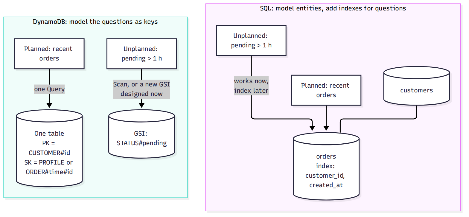
Figure 9. The same feature, two philosophies. In SQL the unplanned question costs a query and maybe an index. In DynamoDB the planned question is one cheap request, and the unplanned one costs a schema change, such as a new GSI (global secondary index, a second copy of the data keyed differently). Which suits you depends on how stable your questions are.

What it costs. DynamoDB's on-demand pricing makes the per-request model concrete. In us-east-1 as of October 2026, AWS lists $0.625 per million write request units (one unit covers a write of up to 1 KB), $0.125 per million read request units (one unit covers a strongly consistent read of up to 4 KB, or two eventually consistent ones), and \(0.25 per GB-month of storage. A steady 1,000 writes a second of items up to 1 KB is about 2.6 billion writes a month, roughly \)1,600. Ten thousand strongly consistent reads a second of items up to 4 KB is about 26 billion reads, roughly $3,300, or half that with eventually consistent reads. At 100,000 writes a second the write bill alone is about $164,000 a month. The price grows in a straight line with traffic, which is wonderful for spiky or small workloads and is the reason steady, very large workloads move to provisioned capacity or to databases they run themselves.

The lines between families have blurred, which is worth knowing before you choose on reputation alone. PostgreSQL stores and indexes JSON documents well with its JSONB type. MongoDB has supported multi-document ACID transactions since version 4.0. DynamoDB has transactions too, limited to 100 items each. The families describe each database's native shape, not a fence around what it can do.

---

Section 5: How each one scales

Scaling a database means handling more data or more traffic than one machine can. There are three main moves, and the order you try them in matters.

Scale up (vertical scaling): a bigger machine. More memory means more of the working set, the data your queries touch regularly, stays in cache, and faster disks mean faster commits. It's the cheapest move in engineering time, and modern servers are big. Its limit is the biggest machine you can buy, and that single machine is still a single point of failure.

Scale reads with replicas: copy the data to read-only replicas and send reads there (#5). This is how OpenAI's single Postgres primary served millions of read queries a second. The catch is replication lag: a replica may be a little behind, so a user who just saved something can read the old version unless you route their reads to the primary for a while.

Pool your connections. In PostgreSQL the first wall is often the number of connections rather than the number of queries. Postgres runs a separate operating-system process for each connection, so thousands of mostly idle connections from autoscaled application servers waste memory, and a burst of new connections can overwhelm the server. OpenAI's 2026 post describes this directly: its managed Postgres had a limit of 5,000 connections per instance, it had incidents from "connection storms that exhausted all available connections," and it put PgBouncer, a connection pooler, in front of every replica. In transaction pooling mode, many client connections share a small number of real database connections, each borrowed only for the length of a transaction; OpenAI reported average connection time dropping from 50 ms to 5 ms. The catch is that anything tied to a session (SET commands, advisory locks, which are locks the application defines for itself, LISTEN, which subscribes a connection to notifications, and temporary tables) doesn't survive moving between real connections, though PgBouncer has supported prepared statements in transaction mode since version 1.21 in 2023.

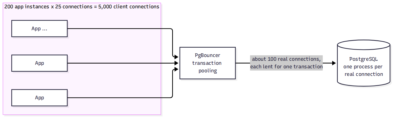
Figure 10. Connection pooling. Without the pooler, every application connection is a Postgres process, mostly sitting idle. With it, thousands of client connections share a pool sized for how many transactions are actually running at once, which is usually a small multiple of the database's CPU cores.

Scale writes by sharding: split the data across several independent databases by a key, so each one holds a slice (#3). This is the only way past one machine's write capacity, and for SQL it's expensive. Queries that join across shards become application code, transactions across shards become the distributed transactions of #15, and moving data between shards becomes an ongoing operational job. That's why so many teams shard only the few tables that need it.

NoSQL systems like DynamoDB, Cassandra, and MongoDB (in sharded mode) have partitioning built in: you choose a partition key and the database spreads data and traffic across machines for you. The work doesn't disappear, though, it moves into choosing the key. A key that sends a large share of traffic to one value creates a hot partition. DynamoDB's documentation, for example, says each partition delivers at most 3,000 read units and 1,000 write units a second (one read unit is one strongly consistent read of up to 4 KB; one write unit is one write of up to 1 KB), so one very popular key hits a ceiling no matter how big the table is.

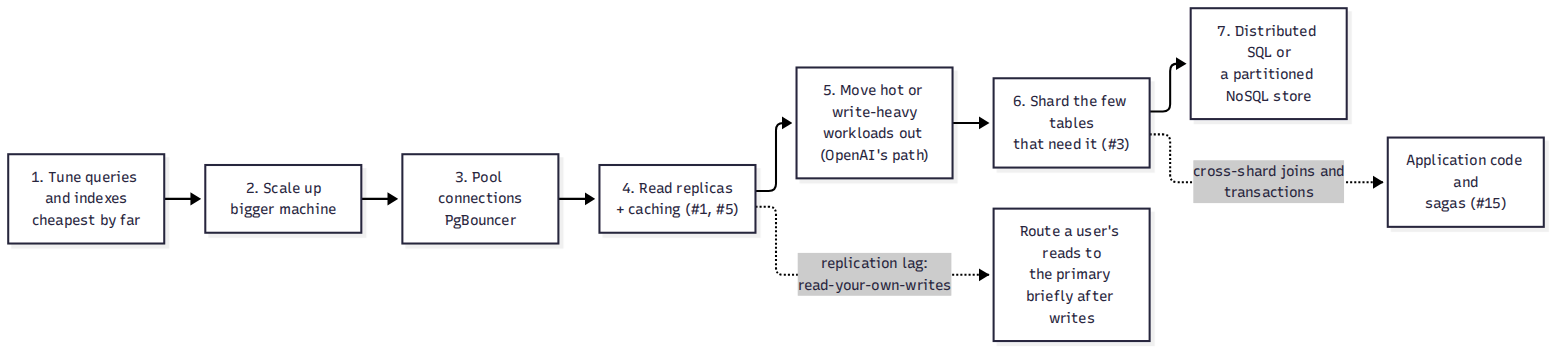
Figure 11. The scaling ladder for a relational database, cheapest step first. Most teams never get past step 4. The dotted arrows are the new problems each step introduces, which is why you climb only as far as measurements force you to.

There's also a middle path. Distributed SQL databases (Google Spanner, CockroachDB, YugabyteDB, TiDB) shard automatically like NoSQL systems while keeping SQL and cross-shard transactions, using replicated consensus groups so a single machine failure doesn't block a commit (#15 explains how). The price is latency, since many writes need agreement across machines and sometimes across regions, along with cost and operational complexity. They're a strong choice when you truly need both relational queries and horizontal write scale.

---

Section 6: CAP, and the more useful question behind it

The famous framing of distributed database tradeoffs is the CAP theorem. Eric Brewer stated it as a conjecture in 2000, and Seth Gilbert and Nancy Lynch proved it in 2002. It says that when a network partition happens, meaning some machines can't reach others, a system replicated across those machines has to choose between:

• Consistency, in a specific sense called linearizability: every read sees the latest completed write, as if there were only one copy of the data.
• Availability: every request to a working machine gets a non-error answer.

On the side of a partition that can't reach the rest, a node can either refuse to answer (keeping consistency) or answer with what it has, which may be stale (keeping availability).

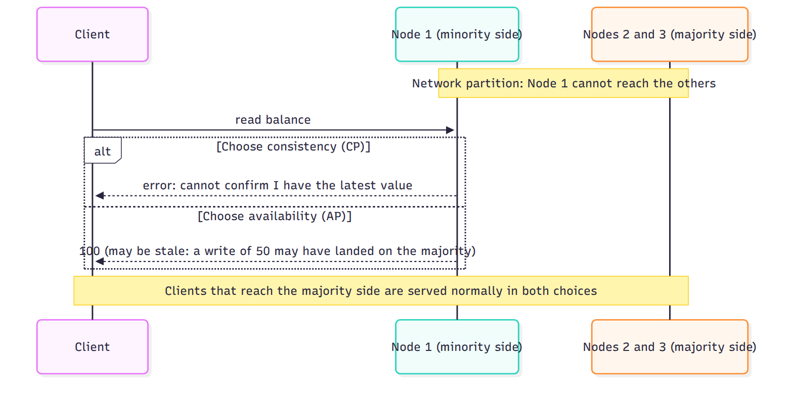
Figure 12. What CAP actually forces. Only the node cut off from the majority faces the choice, and only while the partition lasts: refuse to answer, or answer with what it has. Everyone else carries on, which is why Brewer later called the "pick two of three" framing misleading.

Three corrections to how CAP usually gets explained. First, partitions aren't optional: on real networks they happen, so the choice is never "pick two of three," and Brewer himself wrote in 2012 that the "2 of 3" framing "was always misleading." Second, CAP only describes behavior during a partition. Brewer's same article points out that because partitions are rare, there's little reason to give up consistency or availability the rest of the time. Third, "C" in CAP isn't the "C" in ACID. ACID's consistency is about your declared rules holding; CAP's is about all replicas acting like a single copy.

The more useful framing is PACELC, from Daniel Abadi in 2012: if there's a Partition, choose Availability or Consistency; Else, during normal operation, choose Latency or Consistency. That second half is the tradeoff you live with every day. Waiting for a replica in another region before confirming a write keeps reads consistent everywhere, at the cost of tens of milliseconds on every write.

Real systems let you pick per request. Dynamo-style databases such as Cassandra use quorums: with N copies of each item, a write waits for W replicas to confirm and a read asks R replicas. If R + W > N, every read overlaps at least one replica that saw the latest write, at least in the simple case. Sloppy quorums (writing to substitute replicas during an outage) and last-write-wins conflict resolution based on clocks mean even R + W > N doesn't give linearizability in Dynamo-style stores; Kleppmann's Chapter 5 walks through the edge cases. With N = 3, using W = 2 and R = 2 gives that overlap and tolerates one slow or failed replica; W = 1 and R = 1 is faster but can return stale data. DynamoDB makes the same choice visible in its pricing: a strongly consistent read costs one read unit, and an eventually consistent read costs half that.

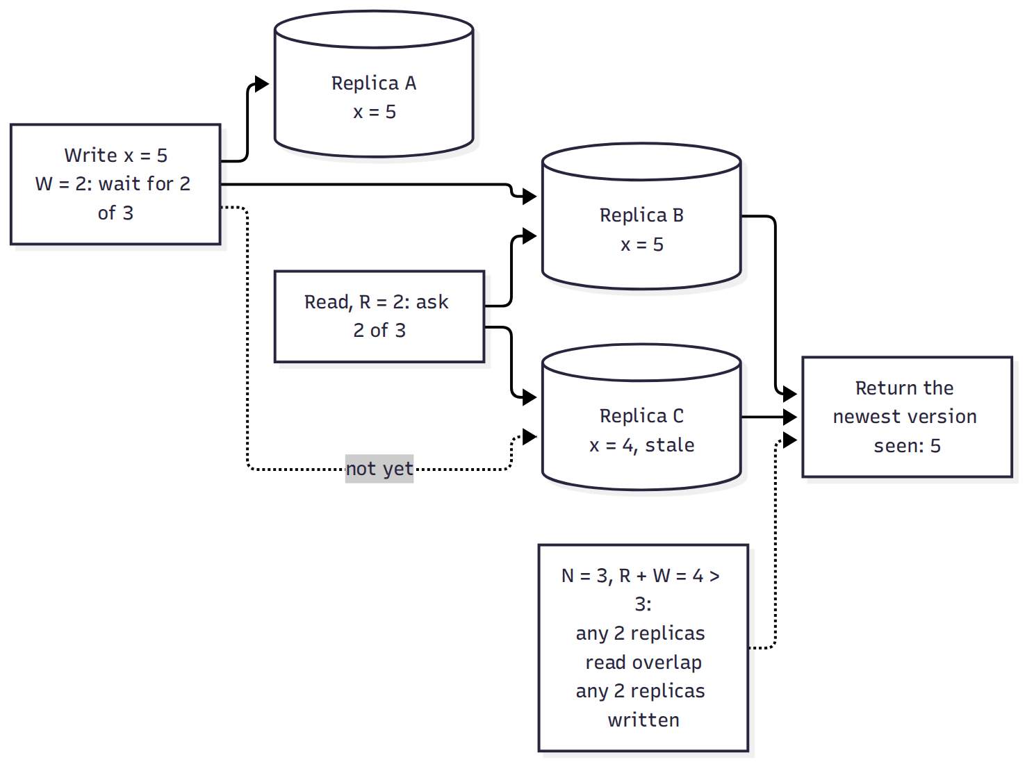
Figure 13. Why R + W > N works in the simple case. With three replicas, any two that acknowledged the write and any two that answer the read must share at least one, so the read sees the new value even though replica C is behind. The caveats in the text (sloppy quorums, clock-based conflict resolution) are the ways real systems break this overlap.

In practice the question becomes: when something breaks, would you rather return a slightly stale answer or an error? A product catalog should serve stale data. A bank balance used to approve a withdrawal should return the error.

---

Section 7: Where each one actually bites

Choosing the right tool is the entry-level skill. Knowing how each tool fails you is the next level, because they all do.

SQL bites at migration time. Changing the schema of a large, busy table is where teams get hurt, and the dangerous part is often the lock, not the work. Modern versions have fixed much of the work: PostgreSQL adds a column with a non-volatile default by storing the default in the table's metadata, without rewriting the table, and MySQL 8.4 adds columns with ALGORITHM=INSTANT by default. But in Postgres, ALTER TABLE still needs a brief ACCESS EXCLUSIVE lock. If a long-running query holds a conflicting lock, the ALTER waits for it, and every new query on that table queues behind the waiting ALTER. A one-millisecond change becomes a full outage of that table. The defense is to set a short lock_timeout and retry, and to run changes as expand-then-contract migrations: add the new column, write to both old and new, backfill in small batches, switch reads over, and only then drop the old column. Each step is safe on its own, and each can be rolled back.

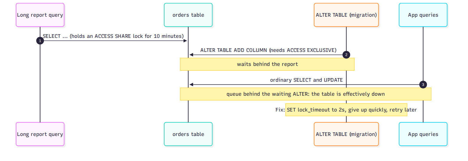
Figure 14. How a one-millisecond schema change causes an outage. The ALTER itself is instant, but it must wait for an exclusive lock, and while it waits every new query on the table queues behind it. A short lock_timeout turns that into a failed migration you retry, instead of a down table.

Figure 15. An expand-then-contract migration. Every numbered step is safe on its own and can be deployed separately, and until step 5 the change can be rolled back by switching reads back, because both columns are still being written. Only the final step is irreversible, and by then nothing uses the old column.

SQL also bites at write scale. Past one primary's write capacity, you're sharding, with the costs from Section 5.

Key-value bites when the questions change. The day the product team asks for "all carts abandoned in the last hour," a design keyed only by cart id has no way to answer except a full scan of the table. The fixes are a secondary index or a second system that maintains one for you, and both cost money and add consistency lag. Model your access patterns before you build, because you can't efficiently query what you didn't plan an index for.

Document stores bite through unbounded growth and shape drift. Embedding a user's entire event history in the user document works until the document approaches the 16-mebibyte limit and every read drags the whole history along. Data that grows without bound belongs in its own collection, referenced by id. And without schema enforcement, "flexible" slowly becomes five services writing five shapes. The fix, schema validation inside the database (MongoDB supports it), means putting back part of what you left SQL to avoid. That's usually the right call anyway.

Wide-column bites through query-first modeling. Newcomers model their entities, then discover the database can't answer their queries without a separate table designed for each access pattern. Cassandra veterans put it simply: model your queries, not your data. Get the queries wrong and you're rebuilding tables under load. Deletes are another surprise: Cassandra marks deleted data with tombstones, markers that are only cleaned up after a grace period, and a query that has to read past many of them gets slow.

Every distributed store bites at the hot key. Whatever the family, all the traffic for one key lands on one partition. A celebrity's profile, a viral post's counter, or a partition key based on the current date will find that ceiling. Design partition keys for an even spread, and plan specifically for the few keys that won't be even (the Twitter/X walkthrough, Design Walkthrough #2, does this in detail).

---

Section 8: The numbers, and a decision framework

Rough orders of magnitude sort designs into buckets. These are not benchmarks: hardware, data size, and query shape move every number. Where a figure has a source, it's named.

System	Rough throughput	Typical latency	Anchor
Redis, one node	about 180,000 simple writes/s unpipelined; over 1.5M with pipelining	sub-millisecond	Redis docs' benchmark examples (one run on a laptop)
PostgreSQL or MySQL, one primary	thousands to tens of thousands of writes/s; tens of thousands or more indexed reads/s	about a millisecond for indexed lookups with hot data in memory	planning bucket; OpenAI ran millions of read QPS with one primary plus about 50 replicas (2026)
DynamoDB	per partition: 3,000 read units, 1,000 write units a second; tables scale by adding partitions	single-digit milliseconds	AWS docs; 151M requests/s peak on Prime Day 2025
Cassandra cluster	about 1.1M client writes/s on 288 nodes, about 3,800 per node	low milliseconds	Netflix benchmark, 2011 hardware
MongoDB, one replica set	similar bucket to one SQL primary; shard to go further	about a millisecond to low milliseconds	planning bucket
Size limits	16 MiB per MongoDB document; 400 KB per DynamoDB item		vendor docs
Postgres connections	5,000 per instance on OpenAI's managed setup; pooled through PgBouncer	50 ms to 5 ms connection time with pooling	OpenAI, 2026
DynamoDB on-demand price	$0.625 per million writes, $0.125 per million reads, $0.25 per GB-month		AWS us-east-1, Oct 2026

If someone tells you their single Postgres primary does a million writes a second, the bucket says to ask questions.

The decision framework, five questions in the order I'd ask them:

1. What questions will you ask? Known keys point to key-value. Ad-hoc questions and joins point to SQL. High-volume time-ordered writes read back by key point to wide-column. Deep relationship traversals point to graph. The access pattern decides more than anything else.
2. How bad is wrong data? Money, inventory, and medical records want ACID transactions, which means SQL or a distributed SQL database, and the right isolation level (Section 3). A like count or a view counter can be eventually consistent.
3. What shape is the data? Uniform records with relationships fit tables. Records with truly varied shapes fit documents (or JSONB inside Postgres). Simple values fetched by id fit key-value.
4. How much write scale, measured rather than imagined? Under roughly 10,000 writes a second, sustained, one SQL primary is usually fine and much simpler. Well past that, across many machines, a database with built-in partitioning or distributed SQL earns its complexity.
5. Who operates it? A managed Postgres you rarely think about beats a self-hosted Cassandra cluster that a team of three can't support around the clock. Operational burden is a real cost, and the most capable database nobody on call understands is the wrong choice.

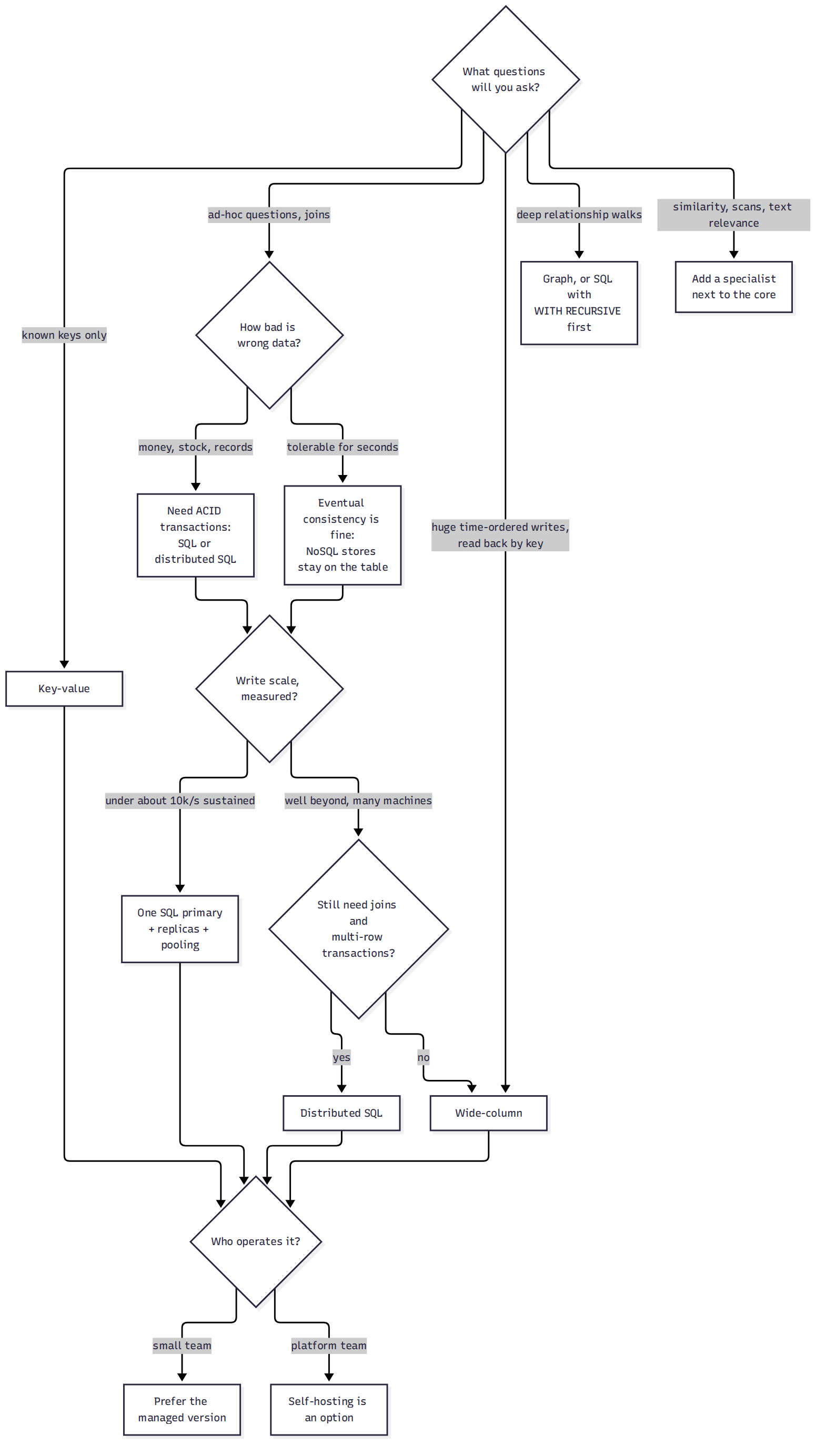
Figure 16. The five questions as a flowchart. Start at the top; most paths land on "one SQL primary" for longer than people expect. The final diamond applies to every choice, because a database nobody on call can operate is the wrong one however well it fits the data.

Work through those and the menu usually narrows to one clear choice and one fallback. Write the fallback down, because requirements change and it's the first draft of your migration plan.

---

Section 9: The principal take: polyglot persistence, and the seams between stores

At most companies of any size, the answer is several databases, each doing what it's good at, an approach called polyglot persistence. A typical system runs PostgreSQL for the transactional core (users, orders, money), Redis for sessions, caches, and rate-limit counters, a search engine such as Elasticsearch or OpenSearch for full-text search, a data warehouse for analytics (the OLAP store from Section 4), and often Kafka as the durable log connecting them.

The principal judgment is knowing where to stop. Every additional database is more operational surface: backups, monitoring, upgrades, security patches, on-call runbooks, and people who know how it fails. The subtler cost lives in the seams between stores. When an order is in Postgres but not yet in the search index, which one is right? If the service writes to Postgres and then to Elasticsearch, a crash between the two leaves them disagreeing forever. That's the dual-write problem from #15, and the fix is the same: write once to the system of record, and feed every other store from its change log (change data capture, or a transactional outbox). Derived stores can then be rebuilt from the log whenever they drift, and every consumer must handle repeats safely (#6).

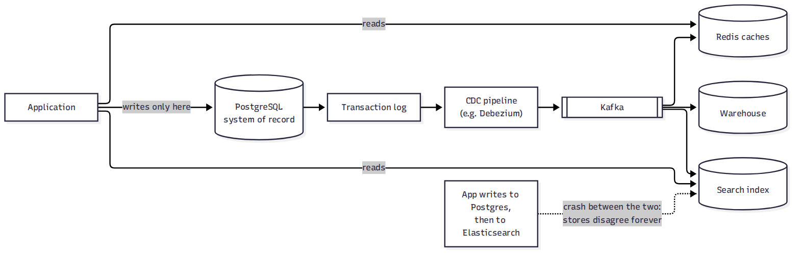
Figure 17. Polyglot persistence without dual writes. The application writes to one place; every other store is fed from that database's own log, so each one can lag but none can permanently disagree, and any of them can be rebuilt by replaying from the log. The dotted path at the bottom is the pattern to avoid.

Moving from one database to another. Section 1 said migrations take months. Here's what fills those months, in the order that keeps every step reversible:

1. Bulk copy, then stream. Take a consistent snapshot of the old database into the new one, then start change data capture from the moment of the snapshot so the new store keeps up with live writes.
2. Verify. Compare row counts and checksums by range, and run shadow reads: serve from the old database, also query the new one, and log every difference.
3. Move reads gradually. Behind a feature flag, send 1%, then 10%, then all reads to the new store, watching latency and the mismatch log.
4. Move writes. This is the hard step. Start reverse CDC, from the new store back to the old one, before the first write lands on the new store, so the old store never falls behind. Then either take a short planned write pause (stop writes, let CDC drain, flip the write target) or, if no pause is acceptable, move writes one slice at a time (by customer or key range), so every record has exactly one writable home at any moment. Avoid having the application write to both stores, for the dual-write reasons from #15.
5. Keep a way back. Leave reverse CDC running for a few weeks, so rolling back is a flag flip rather than another migration.
6. Decommission only after the rollback window passes quietly.

Figure 18. A database migration with a way back at every stage. The dotted arrows are the rollback paths; only the last step removes them. The same shape (copy, verify, ramp, keep the old path warm) is the pull-to-push migration in the Twitter/X walkthrough, applied to storage.

OpenAI's 2026 post is a good model of how this decision should look. They didn't leave PostgreSQL because it was "not web scale." They measured specific pain, write amplification from MVCC, table bloat, and the cost of autovacuum, and they moved only the shardable, write-heavy workloads to a sharded system (Azure Cosmos DB) while keeping Postgres for everything it still does well.

Start with one database, usually PostgreSQL, and add the next only when a measured pain forces it. A latency percentile you can't meet, a write ceiling you've actually hit, or a query the primary can't serve are measurements. "We'll need Cassandra someday" isn't. When you do add a store, decide up front which one is the system of record, how the others are fed from it, and how you'll rebuild them when they drift.

---

The database menu, distilled

Key numbers:

Metric	Value
One Postgres primary at scale	OpenAI: one primary plus nearly 50 replicas, millions of read QPS, 800M users (Jan 2026)
Redis, one node	about 180k simple writes/s unpipelined, 1.5M+ pipelined (Redis docs examples)
DynamoDB partition ceiling	3,000 read units and 1,000 write units a second per partition
DynamoDB at peak	151M requests/s, Prime Day 2025
Cassandra at scale	1.1M client writes/s on 288 nodes, 3.3M with replication (Netflix, 2011)
Document size limits	MongoDB 16 MiB; DynamoDB 400 KB per item
Default isolation	PostgreSQL: read committed. MySQL InnoDB: repeatable read
Quorum overlap rule	R + W > N; with N = 3, R = 2 and W = 2
Rough "one SQL primary is fine" line	under about 10,000 sustained writes a second

Every trade-off, in one table:

Decision	Chose	Over	Why
Default database	PostgreSQL	Starting with NoSQL	ad-hoc queries, transactions, mature tooling; one primary goes far
Isolation	Read committed default, serializable with retries where it matters	Serializable everywhere	throughput for most work, correctness where write skew would hurt
Lost updates	Atomic UPDATE or version checks	Read, modify, write in app code	the app-side version silently loses writes
Known-key access at huge scale	Key-value (DynamoDB, Redis)	SQL	predictable latency; you give up ad-hoc questions
Varied record shapes	Documents or JSONB, with validation	Unvalidated documents	flexibility without five shapes per collection
Massive write volume	Wide-column (Cassandra)	Sharded SQL	built-in partitioning and replication; you model queries, not entities
Relational queries plus write scale	Distributed SQL	Hand-sharded SQL	cross-shard transactions built in; costs latency and money
Schema changes	Expand-then-contract with lock_timeout	One big ALTER	each step safe and reversible; no lock-queue outage
Partition keys	Even spread, plan for hot keys	Natural but skewed keys	one hot key caps the whole table
Consistency level	Per request (quorums, strong vs eventual reads)	One global setting	pay for consistency only where stale data hurts
Multiple stores	One system of record, others fed by CDC	Dual writes from the app	a crash between writes leaves stores disagreeing forever
Adding a database	On measured pain	On predicted future scale	each store adds operational surface and a seam
Vector search	pgvector inside Postgres first	A dedicated vector database first	embeddings next to their rows, filtered with SQL, until scale says otherwise
Analytics	Column store fed by CDC	Heavy reports on the primary	scans of billions of rows belong on a store built for them
Connections	PgBouncer transaction pooling	One real connection per app thread	Postgres runs a process per connection
Database migration	Snapshot + CDC, shadow reads, ramp, reverse CDC	Big-bang cutover	every stage reversible

Three ideas to take with you:

1. The access pattern picks the database. Write down the questions you'll ask, and how often, before comparing databases. Most wrong choices come from choosing by reputation.
2. Know what your guarantees actually are. Your SQL database's default isolation level is probably weaker than you assume, and CAP is about behavior during partitions while PACELC covers the latency you pay every day.
3. Start with one, and add stores carefully. Postgres goes further than its reputation. When you add a second store, make one of them the source of truth and feed the rest from its log.

Further reading

• PostgreSQL: Transaction Isolation. The clearest official explanation of the anomalies, Postgres's three real isolation levels, and serialization failures.
• MySQL: Transaction Isolation Levels. InnoDB's levels and its repeatable-read default.
• Scaling PostgreSQL to power 800 million ChatGPT users. OpenAI, January 2026. How far one primary goes, and the measured reasons they moved write-heavy work elsewhere.
• pgvector. Vector search inside PostgreSQL; the README explains the HNSW and IVFFlat trade-offs.
• DynamoDB data modeling foundations. AWS on single-table versus multiple-table design, with the trade-offs of each.
• PgBouncer 1.21.0 release notes. Prepared-statement support in transaction pooling mode.
• Dynamo: Amazon's Highly Available Key-value Store. DeCandia et al., SOSP 2007. The paper behind quorums, consistent hashing, and much of the NoSQL design that followed.
• Spanner: Google's Globally-Distributed Database. Corbett et al., OSDI 2012. What relational transactions at global scale look like.
• CAP Twelve Years Later: How the "Rules" Have Changed. Eric Brewer, 2012. The theorem's author on what it does and doesn't mean.
• Consistency Tradeoffs in Modern Distributed Database System Design. Daniel Abadi, IEEE Computer, 2012. The PACELC paper.
• Benchmarking Cassandra Scalability on AWS: Over a million writes per second. Netflix Technology Blog, 2011. The 288-node benchmark from Section 4.
• DynamoDB: Designing partition keys. AWS docs on per-partition limits and spreading load evenly.
• Designing Data-Intensive Applications. Martin Kleppmann. In the first edition, Chapter 2 covers data models, Chapter 3 storage engines and indexes, Chapter 5 replication, Chapter 6 partitioning, Chapter 7 transactions and isolation, and Chapter 9 consistency and consensus.

Where you'll meet this

Every system design interview reaches a "which database?" moment, and the strong answer names the access patterns before naming a product. You'll meet these choices in the Twitter/X walkthrough (Design Walkthrough #2): tweets in a store sharded by id, timelines in Redis, search in its own index, all fed from one event stream. And you'll meet them at work in every migration, every new microservice, and every "let's just add Elasticsearch" conversation.

Next up: Core Concepts #17. Until it lands, #15 (distributed transactions) is the natural companion to Section 9 here, since it covers the dual-write fix in depth.

Keep exploring

• Anchor: From Laptop to Billions of Clicks: Designing a URL Shortener in 11 Steps
• Design Walkthrough #2: From One Timeline to 500 Million Tweets a Day: Designing Twitter/X in 11 Steps
• #1 The 100:1 Superpower: Caching
• #2 The Blast Radius: Surviving the Day Your Dependencies Fail
• #3 Divide and Conquer: Sharding and Partitioning
• #4 The Snowflake Problem: Unique IDs at Scale
• #5 Copies of the Truth: Replication
• #6 Do No Harm Twice: Idempotency
• #7 The Copy at the Doorstep: CDNs and Edge Computing
• #8 The Bouncer's Math: Rate Limiting
• #9 What Broke at 3 AM: Observability, p99, and Useful Alerts
• #10 Do It Later, On Purpose: Async Processing and Queues
• #11 The Traffic Cop: Load Balancing
• #12 Assume They're Already Knocking: Security and Abuse at Scale
• #13 Do the Math First: Estimation for System Design
• #14 The Whiteboard Playbook: Taking On Any System Design Challenge
• #15 All or Nothing: Distributed Transactions
• #16 The Database Menu: SQL vs NoSQL (this post)

---

Blueprints of Scale — Core Concepts #16. If this helped, the best thanks is a share with someone who's learning.